Intensity Transformations and Histogram Equalization

The image used for the given intensity transformations is the image below.

---

First it is converted into a grayscale image to apply the intensity transformations. The grayscale of the image is shown below:

---

The results from the intensity transformations that were indicated in the objective are shown as follows.

The first intensity transformation is the image negative which is represented by the equation s = L - 1 – r, where L is the your shifting variable. This image is shown below.

---

The next is your log transform. The pixel values are first converted into double data type. The images below are intensity transformation for log given by the equation s = c log(1 + r) with your c values to be 1 and 4 respectively. By increasing the value of your c, the background seemed to turn lighter revealing a bit more of details. This is because c in the equation is your image’s contrast, increasing it will make your image brighter.

---

Next is the gamma transform, s=crγ. We start from the gray image then we divide the values of this image by 255 in order to give it values less than 1. Then we can utilize a method in opencv, pow, which simply raises the values of the image pixels to the additional supplied numeric parameter.

---

Next are the histogram results from contrast stretching and thresholding.

---

Below is the result for intensity level slicing.

---

The same image was used for histogram equalization. The grayscale image and its histogram is shown below.

---

The cumulative distribution function which is done by getting the cumulative values of your histogram and what the histogram looks like upon equalization is shown below. The resulting image is also shown.

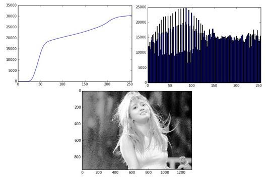
From comparing the initial grayscale image and the one that was applied with histogram equalization, we can that the resulting image turned brighter as well as much more of its details are now visible.